Evaluating Precision in Sports Analytics
One of my data anaylsis pet peeves is false precision. Just because it is possible calculate a quantity to three decimal places doesn’t mean all of those decimal places are meaningful. This post explores how much precision is justified in the context of two common sports statistics: batting average in Major League Baseball and save percentage in the National Hockey League. Using Bayesian hierarchical models, we find that though these quantities are conventionally calculated to three decimal places, only the first two decimal places of precision are justified.
%matplotlib inlineimport arviz as az
from matplotlib import pyplot as plt
from matplotlib.ticker import StrMethodFormatter
import numpy as np
import pandas as pd
import pymc3 as pm
import scipy as sp
import seaborn as snssns.set(color_codes=True)
svpct_formatter = ba_formatter = StrMethodFormatter("{x:.3f}")Batting average
We begin by loading hitting data for the 2018 MLB season from Baseball Reference.
def get_data_url(filename):
    return f"https://www.austinrochford.com/resources/sports_precision/{filename}"
def load_data(filepath, player_col, usecols):
df = pd.read_csv(filepath, usecols=[player_col] + usecols)
return (pd.concat((df[player_col]
.str.split('\\', expand=True)
.rename(columns={0: 'name', 1: 'player_id'}),
df.drop(player_col, axis=1)),
axis=1)
.rename(columns=str.lower)
.groupby(['player_id', 'name'])
.first() # players that switched teams have their entire season stats listed once per team
.reset_index('name'))mlb_df = load_data(get_data_url('2018_batting.csv'), 'Name', ['AB', 'H'])mlb_df.head()| name | ab | h | |
|---|---|---|---|
| player_id | |||
| abreujo02 | Jose Abreu | 499 | 132 |
| acunaro01 | Ronald Acuna | 433 | 127 |
| adamewi01 | Willy Adames | 288 | 80 |
| adamja01 | Jason Adam | 0 | 0 |
| adamsau02 | Austin L. Adams | 0 | 0 |
batter_df = mlb_df[mlb_df['ab'] > 0]
n_player, _ = batter_df.shape
This data set covers nearly 1,000 MLB players.
n_player984Batting average(https://en.wikipedia.org/wiki/Batting_average_(baseball%29) is the most basic summary of a player’s batting performance and is defined as their number of hits divided by their number of at bats. In order to assess the amount of precision that is justified when calculating batting average, we build a hierarchical logistic model. Let \(n_i\) be the number of at bats for the \(i\)-th player and let \(y_i\) be their number of hits. Our model is
\[ \begin{align*} \mu_{\eta} & \sim N(0, 5^2) \\ \sigma_{\eta} & \sim \textrm{Half-}N(2.5^2) \\ \eta_i & \sim N(\mu, \sigma_{\eta}^2) \\ \textrm{ba}_i & = \textrm{sigm}(\eta_i) \\ y_i\ |\ n_i & \sim \textrm{Binomial}(n_i, \textrm{ba}_i). \end{align*} \]
We specify this model in pymc3 below using a non-centered parametrization.
def hierarchical_normal(name, shape, μ=None):
    if μ is None:
        μ = pm.Normal(f"μ_{name}", 0., 5.)

    Δ = pm.Normal(f"Δ_{name}", shape=shape)
    σ = pm.HalfNormal(f"σ_{name}", 2.5)

    return pm.Deterministic(name, μ + Δ * σ)
with pm.Model() as mlb_model:
η = hierarchical_normal("η", n_player)
ba = pm.Deterministic("ba", pm.math.sigmoid(η))
hits = pm.Binomial("hits", batter_df['ab'], ba, observed=batter_df['h'])We proceeed to sample from the model’s posterior distribution.
CHAINS = 3
SEED = 88564 # from random.org, for reproducibility

SAMPLE_KWARGS = {
    'draws': 1000,
    'tune': 1000,
    'chains': CHAINS,
    'cores': CHAINS,
    'random_seed': list(SEED + np.arange(CHAINS))
}
with mlb_model:
mlb_trace = pm.sample(**SAMPLE_KWARGS)Auto-assigning NUTS sampler...
Initializing NUTS using jitter+adapt_diag...
Multiprocess sampling (3 chains in 3 jobs)
NUTS: [σ_η, Δ_η, μ_η]
Sampling 3 chains: 100%|██████████| 6000/6000 [00:44<00:00, 133.94draws/s]Before drawing conclusions from the posterior samples, we use arviz to verify that there are no obvious problems with the sampler diagnostics.
az.plot_energy(mlb_trace);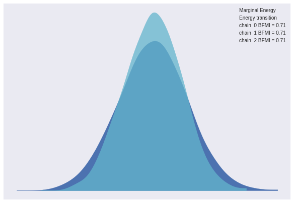
az.gelman_rubin(mlb_trace).max()<xarray.Dataset>
Dimensions: ()
Data variables:
μ_η float64 1.01
Δ_η float64 1.0
σ_η float64 1.0
η float64 1.0
ba float64 1.0First we’ll examine the posterior distribution of Mike Trout’s batting average.
fig, ax = plt.subplots(figsize=(8, 6))

trout_ix = (batter_df.index == 'troutmi01').argmax()
ax.hist(mlb_trace['ba'][:, trout_ix], bins=30, alpha=0.5);

ax.vlines(batter_df['h']
                   .div(batter_df['ab'])
                   .loc['troutmi01'],
          0, 275,
          linestyles='--',
          label="Actual batting average");

ax.xaxis.set_major_formatter(ba_formatter);
ax.set_xlabel("Batting average");

ax.set_ylabel("Posterior density");

ax.legend();
ax.set_title("Mike Trout");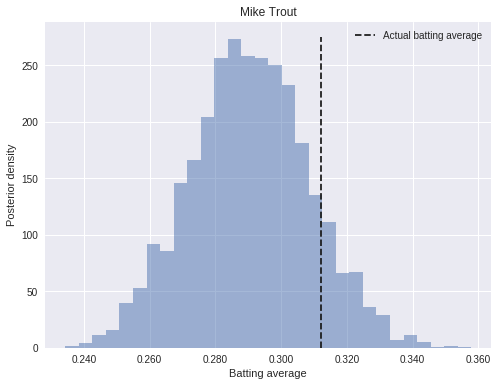
We see that the posterior places significant mass between .260 and .320, quite a wide range of batting averages. This range roughly corresponds to the 95% credible interval for his 2018 batting average.
np.percentile(mlb_trace['ba'][:, trout_ix], [2.5, 97.5])array([ 0.25516468, 0.32704036])We will use the width of the 95% credible interval for each player’s batting average to determine how many digits of precision are justified.
mlb_df = batter_df.assign(
    width_95=sp.stats.iqr(mlb_trace["ba"], axis=0, rng=(2.5, 97.5))
)
The following plot shows the width of these intervals, grouped by the number of at bats the player had in 2018.
def plot_ci_width(grouped, width):
    fig, ax = plt.subplots(figsize=(8, 6))

    low = grouped.quantile(0.025)
    high = grouped.quantile(0.975)

    ax.fill_between(low.index, low, high,
                    alpha=0.25,
                    label=f"{width:.0%} interval");

    grouped.mean().plot(ax=ax, label="Average")

    ax.set_ylabel("Width of 95% credible interval");
    ax.legend(loc=0);

    return ax
ax = plot_ci_width(mlb_df['width_95'].groupby(mlb_df['ab'].round(-2)), 0.95)
ax.set_xlim(0, mlb_df['ab'].max());
ax.set_xlabel("At bats");
ax.set_ylim(bottom=0.);
ax.yaxis.set_major_formatter(ba_formatter);
ax.set_title("Batting average");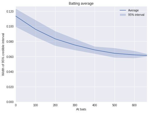
We see that, on average, about 100 at bats are required to justify a single digit of precision in a player’s batting average. Even in the limit of very many at bats (600 at bats corresponds to just under four at bats per game across a 162 game season) the 95% credible interval has an average width approaching 0.060. This limit indicates that batting average is at most meaningful to the second digit, and even the second digit has a fair bit of uncertainty. This result is not surprising; calculating batting average to three decimal places is a historical convention, but I don’t think many analysts rely on the third digit for their decisions/arguments. While intuitive, it is pleasant to have a somewhat rigorous justification for this practice.
Save percentage
We apply a similar analysis to save percentage in the NHL. First we load 2018 goaltending data from Hockey Reference.
nhl_df = load_data(get_data_url('2017_2018_goalies.csv'), 'Player', ['SA', 'SV'])nhl_df.head()| name | sa | sv | |
|---|---|---|---|
| player_id | |||
| allenja01 | Jake Allen | 1614 | 1462 |
| andercr01 | Craig Anderson | 1768 | 1588 |
| anderfr01 | Frederik Andersen | 2211 | 2029 |
| appleke01 | Ken Appleby | 55 | 52 |
| bernijo01 | Jonathan Bernier | 1092 | 997 |
n_goalie, _ = nhl_df.shapeThis data set consists of the goaltending performance of just under 100 players.
n_goalie95Our save percentage model is almost identical to the batting average model. Let \(n_i\) be the number of at shots the \(i\)-th goalie faced and let \(y_i\) be the number of saves they made. The model is
\[ \begin{align*} \mu_{\eta} & \sim N(0, 5^2) \\ \sigma_{\eta} & \sim \textrm{Half-}N(2.5^2) \\ \eta_i & \sim N(\mu, \sigma_{\eta}^2) \\ \textrm{svp}_i & = \textrm{sigm}(\eta_i) \\ y_i\ |\ n_i & \sim \textrm{Binomial}(n_i, \textrm{svp}_i). \end{align*} \]
with pm.Model() as nhl_model:
    η = hierarchical_normal("η", n_goalie)
    svp = pm.Deterministic("svp", pm.math.sigmoid(η))

    saves = pm.Binomial("saves", nhl_df['sa'], svp, observed=nhl_df['sv'])
with nhl_model:
nhl_trace = pm.sample(nuts_kwargs={'target_accept': 0.9}, **SAMPLE_KWARGS)Auto-assigning NUTS sampler...
Initializing NUTS using jitter+adapt_diag...
Multiprocess sampling (3 chains in 3 jobs)
NUTS: [σ_η, Δ_η, μ_η]
Sampling 3 chains: 100%|██████████| 6000/6000 [00:17<00:00, 338.38draws/s]Once again, the convergence diagnostics show no cause for concern.
az.plot_energy(nhl_trace);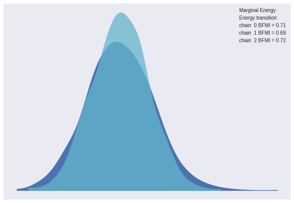
az.gelman_rubin(nhl_trace).max()<xarray.Dataset>
Dimensions: ()
Data variables:
μ_η float64 1.0
Δ_η float64 1.0
σ_η float64 1.0
η float64 1.0
svp float64 1.0We examine the posterior distribution of Sergei Bobrovsky’s save percentage.
fig, ax = plt.subplots(figsize=(8, 6))

bobs_ix = (nhl_df.index == 'bobrose01').argmax()
ax.hist(nhl_trace['svp'][:, bobs_ix], bins=30, alpha=0.5);

ax.vlines(nhl_df['sv']
                .div(nhl_df['sa'])
                .loc['bobrose01'],
          0, 325,
          linestyles='--',
          label="Actual save percentage");

ax.xaxis.set_major_formatter(ba_formatter);
ax.set_xlabel("Save percentage");

ax.set_ylabel("Posterior density");

ax.legend(loc=2);
ax.set_title("Sergei Bobrovsky");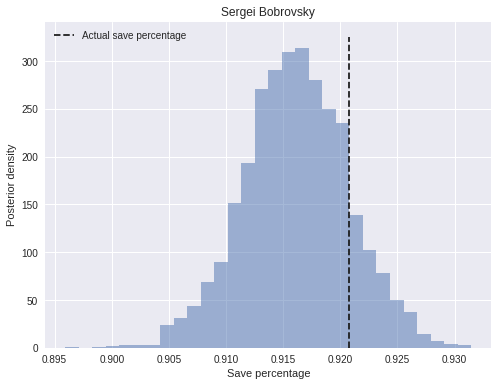
We see that the posterior places significant mass between .905 and .925. We see below that the best and worst save percentages (for goalies that faced at least 200 shots in 2018) are separated by about 0.070.
(nhl_df['sv']
       .div(nhl_df['sa'])
       [nhl_df['sa'] > 200]
       .quantile([0., 1.]))
0.0 0.866995
1.0 0.933712
dtype: float64Sergei Bobrovsky’s 0.020-wide credible interval is a significant proportion of this 0.070 total range.
np.percentile(nhl_trace['svp'][:, bobs_ix], [2.5, 97.5])array([ 0.90683748, 0.92526507])As with batting average, we plot the width of each goalie’s interval, grouped by the number of shots they faced.
nhl_df = nhl_df.assign(
    width_95=sp.stats.iqr(nhl_trace["svp"], axis=0, rng=(2.5, 97.5))
)
ax = plot_ci_width(nhl_df['width_95'].groupby(nhl_df['sa'].round(-2)), 0.95)
ax.set_xlim(0, nhl_df['sa'].max());
ax.set_xlabel("Shots against");
ax.set_ylim(bottom=0.);
ax.yaxis.set_major_formatter(svpct_formatter);
ax.set_title("Save percentage");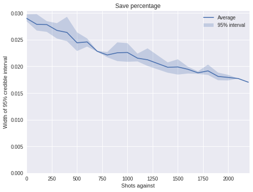
This plot shows that even goalies that face many (2000+) shots have credible intervals wider that 0.010, a signifcant proportion of the total variation between goalies.
This post is available as a Jupyter notebook here.