Stein's Paradox and Empirical Bayes
In mathematical statistics, Stein’s paradox is an important example that shows that an intuitive estimator which is optimal in many senses (maximum likelihood, uniform minimum-variance unbiasedness, best linear unbiasedness, etc.) is not optimal in the most formal, decision-theoretic sense.
This paradox is typically presented from the perspective of frequentist statistics, and this is the perspective from which we present our initial analysis. After the initial discussion, we also present an empirical Bayesian derivation of this estimator. This derivation larely explains the odd form of the estimator and justifies the phenomenon of shrinkage estimators, which, at least to me, have always seemed awkward to justify from the frequentist perpsective. I find the Bayesian perspective on this paradox quite compelling.
A Crash Course in Decision Theory
At its most basic level, statistical decision theory is concerned with quantifying and comparing the effectiveness of various estimators, hypothesis tests, etc. A central concept in this theory is that of a risk function, which is the expected value of the estimator’s error (the loss function). The problem of measuring error appropriately (that is, the choice of an appropriate loss function) is both subtle and deep. In this post, we will only consider the most popular choice, mean squared error,
\[ \begin{align*} MSE(\theta, \hat{\theta}) & = E_\theta \|\theta - \hat{\theta} \|^2. \end{align*} \]
Here \(\theta\) is the parameter we are estimating by \(\hat{\theta}\), and \(\| \cdot \|\) is the Euclidean norm,
\[ \begin{align*} \|\vec{x}\| & = \sqrt{x_1^2 + \cdots + x_n^2}, \end{align*} \]
for \(\vec{x} = (x_1, \ldots x_n)\). Mean squared error is the most widely used risk function because of its simple geometric interpretation and convenient algebraic properties.
While a choice of risk function quantifies the average error of a given estimator, the concept of admissibility provides one framework for comparing different estimators of the same quantity. If \(\Theta\) is the parameter space, we say that the estimator \(\hat{\theta}\) dominates the estimator \(\hat{\eta}\) if
\[ \begin{align*} MSE(\theta, \hat{\theta}) & \leq MSE(\theta, \hat{\eta}) \end{align*} \]
for all \(\theta \in \Theta\), and
\[ \begin{align*} MSE(\theta_0, \hat{\theta}) & < MSE(\theta_0, \hat{\eta}) \end{align*} \]
for some \(\theta_0 \in \Theta\). An estimator is admissible if it is not dominated by any other estimator.
While this definition may feel a bit awkard at first, consider the following example. Suppose that there are only three estimators of \(\theta\), and their mean squared errors are plotted below.
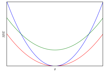
In this diagram, the red estimator dominates both of the other estimators and is admissible.
The James-Stein Estimator
The James-Stein estimator seeks to estimate the mean, \(\theta\) of a multivariate normal distribution, \(N(\theta, \sigma^2 I)\). Here \(I\) is the \(d \times d\) identity matrix, \(\theta\) is an \(d\)-dimensional vector, and \(\sigma^2\) is the known common variance of each component.
If \(X_1 \ldots X_n \sim N(\theta, \sigma^2 I_d)\), the obvious estimator of \(\theta\) is the sample mean, \(\bar{X} = \frac{1}{n} \sum_{i = 1}^n X_i\). This estimator has many nice properties: it is the maximum likelihood estimator of \(\theta\), it is the uniformly minimum-variance unbiased estimator of \(\theta\), it is the best linear unbiased estimator of \(\theta\), it is an efficient estimator of \(\theta\). The James-Stein estimator, however, will show that desipte all of these useful properties, when \(d \geq 3\), the sample mean is an inadmissible estimator of \(\theta\).
The James-Stein estimator of \(\theta\) for the same observations is defined as
\[ \begin{align*} \hat{\theta}_{JS} & = \left( 1 - \frac{(d - 2) \sigma^2}{n \|\bar{X}\|^2} \right) \bar{X}. \end{align*} \]
While the definition of this estimator appears quite strange, it essentially operates by shrinking the sample mean towards zero. The qualifier “essentially” is necessary here, because it is possible, when \(n \| \bar{X} \|^2\) is small relative to \((d - 2) \sigma^2\), that the coefficient on \(\bar{X}\) may be smaller than \(-1\). At the end of our discussion, we will exploit this caveat to show that the James-Stein estimator itself is inadmissible.
We will now prove that the sample mean is inadmissible by calculating the mean squared error of each of these estimators. Using the bias-variance decomposition, we may write the mean squared error of an estimator as
\[ \begin{align*} MSE(\theta, \hat{\theta}) & = \| E_\theta (\hat{\theta}) - \theta \|^2 + tr(Var(\hat{\theta})). \end{align*} \]
We first work with the sample mean. Since this estimator is unbiased, the first term in the decomposition vanishes. It is well known that \(\bar{X} \sim N(\theta, \frac{\sigma^2}{n} I)\). Therefore, the mean squared error for the sample mean is
\[ \begin{align*} MSE(\theta, \bar{X}) & = \frac{d \sigma^2}{n}. \end{align*} \]
The mean squared error of the James-Stein estimator is given by
\[ \begin{align*} MSE(\theta, \hat{\theta}_{JS}) & = \frac{d \sigma^2}{n} - \frac{(d - 2)^2 \sigma^4}{n^2} E_\theta \left( \frac{1}{\| \bar{X} \|^2} \right). \end{align*} \]
Unfortunately, the derivation of this expression is too involved to reproduce here. For details of this derivation, consult Lehmann and Casella1.
We see immediately that the first term of this expression is the mean squared error of the sample mean. Therefore, as long as \(E_\theta (\| \bar{X} \|^{-2})\) is finite, the James-Stein estimator will dominate the sample mean. Note that since \(\theta = 0\) will lead to the smallest sample mean on average, \(E_\theta (\| \bar{X} \|^{-2}) \leq E_0 (\| \bar{X} \|^{-2})\). When \(\theta = 0\), \(\| \bar{X} \|^{-2}\) has an inverse chi-squared distribution with \(d\) degrees of freedom. The mean of an inverse chi-squared random variable is finite if and only if there are at least three degrees of freedom, so we see that for \(d \geq 3\),
\[ \begin{align*} MSE(\theta, \hat{\theta}_{JS}) & \leq \frac{d \sigma^2}{n} - \frac{(d - 2)^2 \sigma^4}{n^2} E_0 \left( \frac{1}{\| \bar{X} \|^2} \right) \\ & = \frac{d \sigma^2}{n} - \frac{(d - 2)^2 \sigma^4}{n^2} \left( \frac{1}{d - 2} \right) \\ & = \frac{d \sigma^2}{n} - \frac{(d - 2) \sigma^4}{n^2}, \end{align*} \]
so the James-Stein estimator dominates the sample mean, and the sample mean is therefore inadmissible.
The natural question now is whether or not the James-Stein estimator is admissible; it is not. As we previously observed, when \(\| \bar{X} \|\) is small enough, the coefficient in the James-Stein estimator may be smaller than \(-1\), and, in this case, it is not shrinking \(\bar{X}\) towards zero. We may remedy this problem by defining a modified James-Stein estimator,
\[ \begin{align*} \hat{\theta}_{JS'} & = \operatorname{max} \left\{ 0, 1 - \frac{(d - 2) \sigma^2}{n \|\bar{X}\|^2} \right\} \cdot \bar{X}. \end{align*} \]
It can be shown that this estimator has smaller mean squared error than the James-Stein estimator. This modification amounts to estimating the mean as zero when \(\| \bar{X} \|\) is small enough to cause a negative coefficient, which is reminiscent of Hodge’s estimator. This modified James-Stein estimator is also not admissible, but we will not discuss why here.
Empirical Bayes and the James-Stein Estimator
The benefits of shrinkage are an interesting topic, but not immediately obvious. To me, the derivation of the James-Stein estimator using the empirical Bayes method illuminates this topic nicely and relates it to a fundamental tenet of Bayesian statistics.
As before, we are attempting to estimate the mean of the distribution \(N(\theta, \sigma^2 I)\) with known variance \(\sigma^2\) from samples \(X_1, \ldots, X_n\). To do so, we place a \(N(0, \tau^2 I)\) prior distribution on \(\theta\). Combining these prior and sampling distributions gives the posterior distribution
\[ \begin{align*} \theta | X_1, \ldots, X_n & \sim N \left( \frac{\tau^2}{\frac{\sigma^2}{n} + \tau^2} \cdot \bar{X}, \left(\frac{1}{\tau^2} + \frac{n}{\sigma^2}\right)^{-1} \right) \end{align*} \]
So the Bayes estimator of \(\theta\) is
\[ \begin{align*} \hat{\theta}_{Bayes} & = E(\theta | X_1, \ldots, X_n) = \frac{\tau^2}{\frac{\sigma^2}{n} + \tau^2} \cdot \bar{X}. \end{align*} \]
The value of \(\sigma^2\) is known, but, in general, we do not know the value of \(\tau^2\). We will now estimate \(\tau^2\) from the data \(X_1, \ldots, X_n\). This estimation of the hyperparameter \(\tau^2\) from the data is what causes this approach to be empirical Bayesian, and not fully Bayesian. The difference between the fully Bayesian and empirical Bayesian approach is interesting both philosophically and decision-theoretically. Its practicality here is that it often allows us to more easily produce estimators that approximate fully Bayesian estimators with similar (though slightly worse) properties.
There are many ways to approach this problem within the empirical Bayes framework. The James-Stein estimator arises from this situation when we find an unbiased estimator of the coefficient in the definition of \(\hat{\theta}_{Bayes}\). First, we note that the marginal distribution of \(\bar{X}\) is \(N(0, (\frac{\sigma^2}{n} + \tau^2) I)\). We can use this fact to show that
\[ \begin{align*} \frac{\frac{\sigma^2}{n} + \tau^2}{\| \bar{X} \|^2} & \sim \textrm{Inv-}\chi^2 (d). \end{align*} \]
Since the mean of an inverse chi-squared distributed random variables with \(d \geq 3\) degrees of freedom is \(\frac{1}{d - 2}\), we get that
\[ \begin{align*} E \left(1 - \frac{(d - 2) \sigma^2}{n \| \bar{X} \|^2}\right) & = \frac{\tau^2}{\frac{\sigma^2}{n} + \tau^2}. \end{align*} \]
We therefore see that the empirical Bayes method, combined with unbiased estimation yields the James-Stein estimator.
To me, this derivation more clearly explains the phenomenon of shrinkage. Bayes estimators may often be seen as a weighted sum of the prior information, in this case, that the mean was likely to be close to zero, and the evidence, the observed values of \(X\). In this context, it makes much more sense that an estimator which shrinks its estimate toward zero seem well-justified.
Lehmann, E. L.; Casella, G. (1998), Theory of Point Estimation (2nd ed.), Springer↩︎