Bayesian Hypothesis Testing with PyMC

Lately I’ve been reading the excellent, open source book Probabilistic Programming and Bayesian Methods for Hackers. The book’s prologue opens with the following line.

The Bayesian method is the natural approach to inference, yet it is hidden from readers behind chapters of slow, mathematical analysis.

As a mathematician with training in statistics as well, this comment rings quite true. Even with a firm foundation in the probability theory necessary for Bayesian inference, the calculations involved are often incredibly tedious. An introduction to Bayesian statistics often invovles the hazing ritual of showing that, if \(X | \mu \sim N(\mu, \sigma^2)\) and \(\mu \sim N(\mu_0, \sigma_0^2)\) where \(\sigma^2\), \(\mu_0\), and \(\sigma_0^2\) are known, then

\[\mu | X \sim N \left(\frac{\frac{X}{\sigma^2} + \frac{\mu_0}{\sigma_0^2}}{\frac{1}{\sigma^2} + \frac{1}{\sigma_0^2}}\right).\]

If you want to try it yourself, Bayes' Theorem and this polynomial identity will prove helpful.

Programming and Bayesian Methods for Hackers emphasizes the utility of PyMC for both eliminating tedious, error-prone calculations, and also for approximating posterior distributions in models that have no exact solution. I was recently reminded of PyMC’s ability to eliminate tedious, error-prone calculations during my statistics final, which contained a problem on Bayesian hypothesis testing. This post aims to present both the exact theoretical analysis of this problem and its approximate solution using PyMC.

The problem is as follows.

Given that \(X | \mu \sim N(\mu, \sigma^2)\), where \(\sigma^2\) is known, we wish to test the hypothesis \(H_0: \mu = 0\) vs. \(H_A: \mu \neq 0\). To do so in a Bayesian framework, we need prior probabilities on each of the hypotheses and a distribution on the parameter space of the alternative hypothesis. We assign the hypotheses equal prior probabilities, \(\pi_0 = \frac{1}{2} = \pi_A\), which indicates that prior to observing the value of \(X\), we believe that each hypothesis is equally likely to be true. We also endow the alternative parameter space, \(\Theta_A = (-\infty, 0) \cup (0, \infty)\), with a \(N(0, \sigma_0^2)\) distribution, where \(\sigma_0^2\) is known.

The Bayesian framework for hypothesis testing relies on the calculation of the posterior odds of the hypotheses,

\[\textrm{Odds}(H_A|x) = \frac{P(H_A | x)}{P(H_0 | x)} = BF(x) \cdot \frac{\pi_A}{\pi_0},\]

where \(BF(x)\) is the Bayes factor. In our situation, the Bayes factor is

\[BF(x) = \frac{\int_{\Theta_A} f(x|\mu) \rho_A(\mu)\ d\mu}{f(x|0)}.\]

The Bayes factor is the Bayesian counterpart of the likelihood ratio, which is ubiquitous in frequentist hypothesis testing. The idea behind Bayesian hypothesis testing is that we should choose whichever hypothesis better explains the observation, so we reject \(H_0\) when \(\textrm{Odds}(H_A) > 1\), and accept \(H_0\) otherwise. In our situation, \(\pi_0 = \frac{1}{2} = \pi_A\), so \(\textrm{Odds}(H_A) = BF(x)\). Therefore we base our decision on the value of the Bayes factor.

In the following sections, we calculate this Bayes factor exactly and approximate it with PyMC. If you’re only interested in the simulation and would like to skip the exact calculation (I can’t blame you) go straight to the section on PyMC approximation.

Exact Calculation

The calculation becomes (somewhat) simpler if we reparamatrize the normal distribution using its precision instead of its variance. If \(X\) is normally distributed with variance \(\sigma^2\), its precision is \(\tau = \frac{1}{\sigma^2}\). When a normal distribution is parametrized by precision, its probability density function is

\[f(x|\mu, \tau) = \sqrt{\frac{\tau}{2 \pi}} \textrm{exp}\left(-\frac{\tau}{2} (x - \mu)^2\right).\]

Reparametrizing the problem in this way, we get \(\tau = \frac{1}{\sigma^2}\) and \(\tau_0 = \frac{1}{\sigma_0^2}\), so

\[\begin{align} f(x|\mu) \rho_A(\mu) & = \left(\sqrt{\frac{\tau}{2 \pi}} \textrm{exp}\left(-\frac{\tau}{2} (x - \mu)^2\right)\right) \cdot \left(\sqrt{\frac{\tau_0}{2 \pi}} \textrm{exp}\left(-\frac{\tau_0}{2} \mu^2\right)\right) \\ & = \frac{\sqrt{\tau \cdot \tau_0}}{2 \pi} \cdot \textrm{exp} \left(-\frac{1}{2} \left(\tau (x - \mu)^2 + \tau_0 \mu^2\right)\right). \end{align}\]

Focusing momentarily on the sum of quadratics in the exponent, we rewrite it as \[\begin{align} \tau (x - \mu)^2 + \tau_0 \mu^2 & = \tau x^2 + (\tau + \tau_0) \left(\mu^2 - 2 \frac{\tau}{\tau + \tau_0} \mu x\right) \\ & = \tau x^2 + (\tau + \tau_0) \left(\left(\mu - \frac{\tau}{\tau + \tau_0} x\right)^2 - \left(\frac{\tau}{\tau + \tau_0}\right)^2 x^2\right) \\ & = \left(\tau - \frac{\tau^2}{\tau + \tau_0}\right) x^2 + (\tau + \tau_0) \left(\mu - \frac{\tau}{\tau + \tau_0} x\right)^2 \\ & = \frac{\tau \tau_0}{\tau + \tau_0} x^2 + (\tau + \tau_0) \left(\mu - \frac{\tau}{\tau + \tau_0} x\right)^2. \end{align}\]

Therefore \[\begin{align} \int_{\Theta_A} f(x|\mu) \rho_A(\mu)\ d\mu & = \frac{\sqrt{\tau \tau_0}}{2 \pi} \cdot \textrm{exp}\left(-\frac{1}{2} \left(\frac{\tau \tau_0}{\tau + \tau_0}\right) x^2\right) \int_{-\infty}^\infty \textrm{exp}\left(-\frac{1}{2} (\tau + \tau_0) \left(\mu - \frac{\tau}{\tau + \tau_0} x\right)^2\right)\ d\mu \\ & = \frac{\sqrt{\tau \tau_0}}{2 \pi} \cdot \textrm{exp}\left(-\frac{1}{2} \left(\frac{\tau \tau_0}{\tau + \tau_0}\right) x^2\right) \cdot \sqrt{\frac{2 \pi}{\tau + \tau_0}} \\ & = \frac{1}{\sqrt{2 \pi}} \cdot \sqrt{\frac{\tau \tau_0}{\tau + \tau_0}} \cdot \textrm{exp}\left(-\frac{1}{2} \left(\frac{\tau \tau_0}{\tau + \tau_0}\right) x^2\right). \end{align}\]

The denominator of the Bayes factor is \[\begin{align} f(x|0) & = \sqrt{\frac{\tau}{2 \pi}} \cdot \textrm{exp}\left(-\frac{\tau}{2} x^2\right), \end{align}\] so the Bayes factor is \[\begin{align} BF(x) & = \frac{\frac{1}{\sqrt{2 \pi}} \cdot \sqrt{\frac{\tau \tau_0}{\tau + \tau_0}} \cdot \textrm{exp}\left(-\frac{1}{2} \left(\frac{\tau \tau_0}{\tau + \tau_0}\right) x^2\right)}{\sqrt{\frac{\tau}{2 \pi}} \cdot \textrm{exp}\left(-\frac{\tau}{2} x^2\right)} \\ & = \sqrt{\frac{\tau_0}{\tau + \tau_0}} \cdot \textrm{exp}\left(-\frac{\tau}{2} \left(\frac{\tau_0}{\tau + \tau_0} - 1\right) x^2\right) \\ & = \sqrt{\frac{\tau_0}{\tau + \tau_0}} \cdot \textrm{exp}\left(\frac{1}{2} \left(\frac{\tau^2}{\tau + \tau_0}\right) x^2\right). \end{align}\]

From above, we reject the null hypothesis whenever \(BF(x) > 1\), which is equivalent to \[\begin{align} \textrm{exp}\left(\frac{1}{2} \left(\frac{\tau^2}{\tau + \tau_0}\right) x^2\right) & > \sqrt{\frac{\tau + \tau_0}{\tau_0}}, \\ \frac{1}{2} \left(\frac{\tau^2}{\tau + \tau_0}\right) x^2 & > \frac{1}{2} \log\left(\frac{\tau + \tau_0}{\tau_0}\right),\textrm{ and} \\ x^2 & > \left(\frac{\tau + \tau_0}{\tau^2}\right) \cdot \log\left(\frac{\tau + \tau_0}{\tau_0}\right). \end{align}\]

As you can see, this calculation is no fun. I’ve even left out a lot of details that are only really clear once you’ve done this sort of calculation many times. Let’s see how PyMC can help us avoid this tedium.

PyMC Approximation

PyMC is a Python module that uses Markov chain Monte Carlo methods (and others) to fit Bayesian statistical models. If you’re unfamiliar with Markov chains, Monte Carlo methods, or Markov chain Monte Carlo methods, each of which is a an important topic in its own right, PyMC provides a set of tools to approximate marginal and posterior distributions of Bayesian statistical models.

To solve this problem, we will use PyMC to approximate \(\int_{\Theta_A} f(x|\mu) \rho_A(\mu)\ d\mu\), the numerator of the Bayes factor. This quantity is the marginal distribution of the observation, \(X\), under the alternative hypothesis.

We begin by importing the necessary Python packages.

import numpy as np
import pymc
import scipy.optimize as opt
import scipy.stats as stats

In order to use PyMC to approximate the Bayes factor, we must fix numeric values of \(\sigma^2\) and \(\sigma_0^2\). We use the values \(\sigma^2 = 1\) and \(\sigma_0^2 = 9\).

simga = 1.0
tau = 1 / sigma**2

sigma0 = 3.0
tau0 = 1 / sigma0**2

We now initialize the random variable \(\mu\).

mu = pymc.Normal("mu", mu=0, tau=tau0)

Note that PyMC’s normal distribution is parametrized in terms of the precision and not the variance. When we initialize the variable x, we use the variable mu as its mean.

x = pymc.Normal("x", mu=mu, tau=tau)

PyMC now knows that the distribution of x depends on the value of mu and will respect this relationship in its simulation.

We now instantiate a Markov chain Monte Carlo sampler, and use it to sample from the distributions of mu and x.

mcmc = pymc.MCMC([mu, x])
mcmc.sample(50000, 10000, 1)

In the second line above, we tell PyMC to run the Markov chain Monte Carlo simulation for 50,000 steps, using the first 10,000 steps as burn-in, and then count each o the last 40,000 steps towards the sample. The burn-in period is the number of samples we discard from the beginning of the Markov chain Monte Carlo algorithm. A burn-in period is necessary to assure that the algorithm has converged to the desired distribution before we sample from it.

Finally, we may obtain samples from the distribution of \(X\) under the alternative hypothesis.

x_samples = mcmc.trace("x")[:]

From our exact calculations, we expect that, given the alternative hypothesis, \(X \sim N\left(0, \frac{\tau \tau_0}{\tau + \tau_0}\right)\). The following chart shows both the histogram derived from x_samples and the probability density function of \(X\) under the alternative hypothesis.

fig = plt.figure(figsize=(5,5))
axes = fig.add_subplot(111)
axes.hist(x_samples, bins=50, normed=True, color="gray");
x_range = np.arange(-15, 15, 0.1)
x_precision = tau * tau0 / (tau + tau0)
axes.plot(x_range, stats.norm.pdf(x_range, 0, 1 / sqrt(x_precision)), color='k', linewidth=2);
fig.show()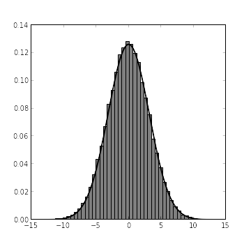

It’s always nice to see agreement between theory and simulation. The problem now is that we need to evaluate the probability distribution function of \(X|H_A\) at the observed point \(X = x_0\), but we only know the cumulative distribution function of \(X\) (via its histogram, computed from x_samples). Enter kernel density estimation, a nonparametric method for estimating the probability density function of a random variable from samples. Fortunately, SciPy provides an excellent module for kernel density estimation.

x_pdf = stats.kde.gaussian_kde(x_samples)

We define two functions, the first of which gives the simulated Bayes factor, and the second of which gives the exact Bayes factor.

def bayes_factor_sim(x_obs):
    return x_pdf.evaluate(x_obs) / stats.norm.pdf(x_obs, 0, sigma)

def bayes_factor_exact(x_obs):
    return sqrt(tau0 / (tau + tau0)) * exp(0.5 * tau**2 / (tau + tau0) * x_obs**2)

The following figure shows the excellent agreement between the simulated and calculated bayes factors.

fig = plt.figure(figsize=(5,5))
axes = fig.add_subplot(111)
x_range = np.arange(0, 2, 0.1)
axes.plot(x_range, bayes_factor_sim(x_range), color="red", label="Simulated Bayes factor", linewidth=2)
axes.plot(x_range, bayes_factor_exact(x_range), color="blue", label="Exact Bayes factor")
axes.legend(loc=2)
fig.show()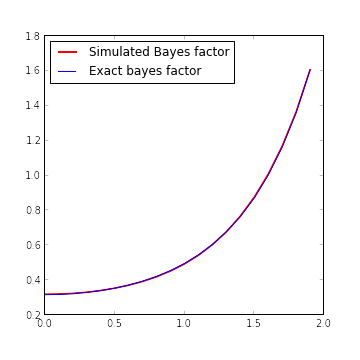

The only reason it’s possible to see the red graph of simulated Bayes factor behind the blue graph of the exact Bayes factor is that we’ve doubled the width of the red graph. In fact, on the interval \([0, 2]\), the maximum relative error of the simulated Bayes factor is approximately 0.9%.

np.max(np.abs(bayes_factor_sim(x_factor_range) - bayes_factor_exact(x_factor_range)) / bayes_factor_exact(x_factor_range))
> 0.0087099167640844726

We now use the simulated Bayes factor to approximate the critical value for rejecting the null hypothesis.

def bayes_factor_crit_helper(x):
    return bayes_factor_sim(x) - 1

x_crit = opt.brentq(bayes_factor_crit_helper, 0, 2)
x_crit
> 1.5949702067681601

The SciPy function opt.brentq is used to find a solution of the equation bayes_factor_sim(x) = 1, which is equivalent to finding a zero of bayes_factor_crit_helper. We plug x_crit into bayes_factor_exact in order to verify that we have, in fact, found the critical value.

bayes_factor_exact(x_crit)
> 0.99349717121979564

This value is quite close to one, so we have in fact approximated the critical point well.

It’s interesting to note that we have used PyMC in a somewhat odd way here, to approximate the marginal distribution of \(X\) under the null hypothesis. A much more typical use of PyMC and its Markov chain Monte Carlo would be to fix an observed value of \(X\) and approximate the posterior distribution of \(\mu\) given this observation.