The HMC Revolution is Open Source¶

Probabilistic Programming with PyMC3¶

@AustinRochford • Tom Tom AMLC • Charlottesville • 4/11/19¶

Who am I?¶

PyMC3 developer • Chief Data Scientist @ Monetate ¶

@AustinRochford • Website • GitHub ¶

arochford@monetate.com • austin.rochford@gmail.com ¶

About This Talk¶

About Monetate¶

Founded 2008, web optimization and personalization SaaS
Observed 5B impressions and $4.1B in revenue during Cyber Week 2017

monetate.com/about/careers

Modern Bayesian Inference¶

Motivating Examples¶

2017 UK General Election¶

Source

NBA Foul Calls¶

Source

Player skills(?)¶

Probabilistic Programming¶

Data Science — inference enables storytelling

Probabilistic Programming — storytelling enables inference

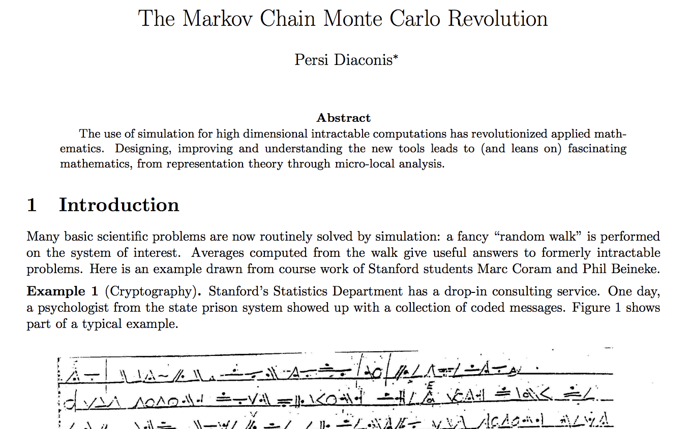
The Monty Hall Problem¶

Initially, we have no information about which door the prize is behind.

In [8]:

import pymc3 as pm

with pm.Model() as monty_model:
    prize = pm.DiscreteUniform('prize', 0, 2)

If we choose door one:

	Monty can open
Prize behind	Door 1	Door 2	Door 3
Door 1	No	Yes	Yes
Door 2	No	No	Yes
Door 3	No	Yes	No

In [9]:

from theano import tensor as tt

with monty_model:
    p_open = pm.Deterministic(
        'p_open',
        tt.switch(tt.eq(prize, 0),
            np.array([0., 0.5, 0.5]), # it is behind the first door
        tt.switch(tt.eq(prize, 1),
            np.array([0., 0., 1.]),   # it is behind the second door
            np.array([0., 1., 0.])))  # it is behind the third door
    )

Monty opened the third door, revealing a goat.

In [10]:

with monty_model:
    opened = pm.Categorical('opened', p_open, observed=2)

Should we switch our choice of door?

In [13]:

with monty_model:
    monty_trace = pm.sample(1000, **MONTY_SAMPLE_KWARGS)
    
monty_df = pm.trace_to_dataframe(monty_trace)

Multiprocess sampling (3 chains in 3 jobs)
Metropolis: [prize]
Sampling 3 chains: 100%|██████████| 4500/4500 [00:01<00:00, 4173.25draws/s]

In [14]:

monty_df['prize'].head()

Out[14]:

0    0
1    0
2    0
3    0
4    1
Name: prize, dtype: int64

In [15]:

ax = (monty_df['prize']
              .value_counts(normalize=True, ascending=True)
              .plot(kind='bar', color='C0'))

ax.set_xlabel("Door");
ax.yaxis.set_major_formatter(pct_formatter);
ax.set_ylabel("Probability of prize");

From the PyMC3 documentation:

PyMC3 is a Python package for Bayesian statistical modeling and Probabilistic Machine Learning which focuses on advanced Markov chain Monte Carlo and variational fitting algorithms. Its flexibility and extensibility make it applicable to a large suite of problems.

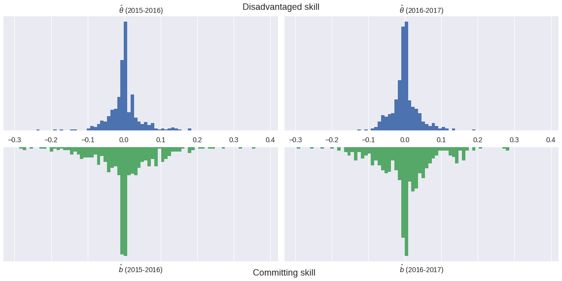
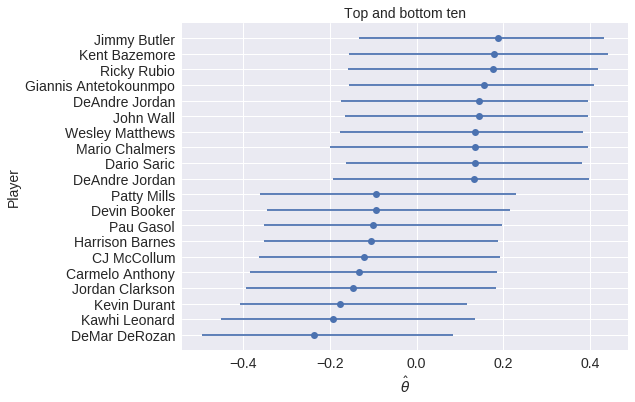
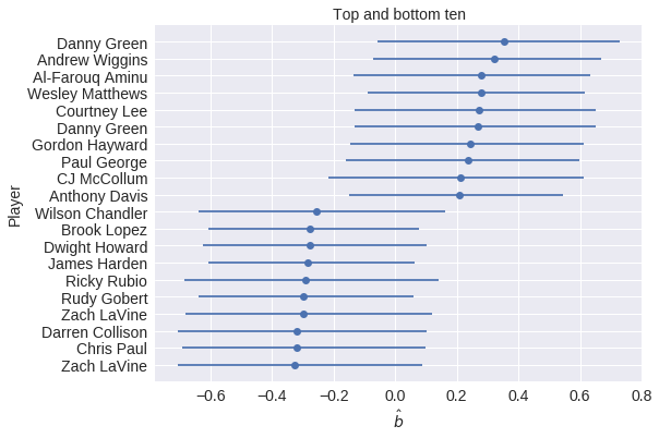
Case Study: NBA Foul Calls¶

Question: Is (not) committing and/or drawing fouls a measurable player skill?

In [19]:

orig_df.head(n=2).T

Out[19]:

play_id	20150301CLEHOU-0	20150301CLEHOU-1
period	Q4	Q4
seconds_left	112	103
call_type	Foul: Shooting	Foul: Shooting
committing_player	Josh Smith	J.R. Smith
disadvantaged_player	Kevin Love	James Harden
review_decision	CNC	CC
away	CLE	CLE
home	HOU	HOU
date	2015-03-01 00:00:00	2015-03-01 00:00:00
score_away	103	103
score_home	105	105
disadvantaged_team	CLE	HOU
committing_team	HOU	CLE

Model outline¶

$$ \operatorname{log-odds}(\textrm{Foul}) \ \sim \textrm{Season factor} + \left(\textrm{Disadvantaged skill} - \textrm{Committing skill}\right) $$

In [29]:

with pm.Model() as irt_model:
    β_season = pm.Normal('β_season', 0., 2.5, shape=n_season)
    
    θ = hierarchical_normal('θ', n_player) # disadvantaged skill
    b = hierarchical_normal('b', n_player) # committing skill

    p = pm.math.sigmoid(
        β_season[season] + θ[player_disadvantaged] - b[player_committing]
    )
    
    obs = pm.Bernoulli(
        'obs', p,
        observed=df['foul_called'].values
    )

Metropolis-Hastings Inference¶

In [30]:

with irt_model: 
    step = pm.Metropolis()
    met_trace = pm.sample(5000, step=step, **SAMPLE_KWARGS)

Multiprocess sampling (3 chains in 3 jobs)
CompoundStep
>Metropolis: [σ_b]
>Metropolis: [Δ_b]
>Metropolis: [σ_θ]
>Metropolis: [Δ_θ]
>Metropolis: [β_season]
Sampling 3 chains: 100%|██████████| 16500/16500 [01:48<00:00, 152.44draws/s]
The gelman-rubin statistic is larger than 1.4 for some parameters. The sampler did not converge.
The estimated number of effective samples is smaller than 200 for some parameters.

In [33]:

trace_fig

Out[33]:

In [34]:

max(np.max(var_stats) for var_stats in pm.gelman_rubin(met_trace).values())

Out[34]:

3.1038666861280597

The Curse of Dimensionality¶

This model has

In [35]:

n_param = n_season + 2 * n_player
n_param

Out[35]:

parameters

In [38]:

fig

Out[38]:

Hamiltonian Monte Carlo Inference¶

Bayesian inference ⇔ Differential geometry¶

Case Study Continued: NBA Foul Calls¶

In [39]:

with irt_model:
    nuts_trace = pm.sample(500, **SAMPLE_KWARGS)

Auto-assigning NUTS sampler...
Initializing NUTS using jitter+adapt_diag...
Multiprocess sampling (3 chains in 3 jobs)
NUTS: [σ_b, Δ_b, σ_θ, Δ_θ, β_season]
Sampling 3 chains: 100%|██████████| 3000/3000 [02:14<00:00, 22.23draws/s]

In [40]:

nuts_gr_stats = pm.gelman_rubin(nuts_trace)
max(np.max(var_stats) for var_stats in nuts_gr_stats.values())

Out[40]:

1.0069298341016355

In [43]:

fig

Out[43]:

Basketball strategy leads to more complexity¶

In [48]:

fig

Out[48]:

Next Steps with Probabilistic Programming¶

PyMC3¶

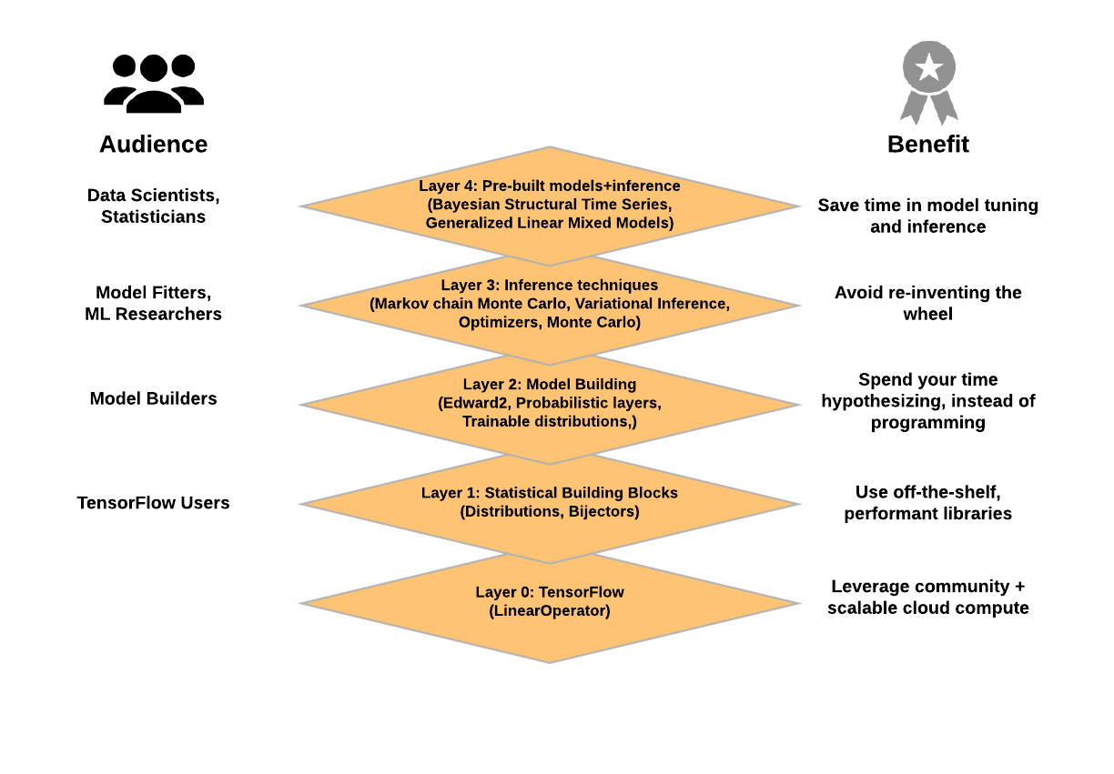
Probabilistic Programming Ecosystem¶

PyMC4?¶

TensorFlow Probability

Prototype repository

Hamiltonian Monte Carlo¶

A Conceptual Introduction to Hamiltonian Monte Carlo

Thank you!¶