Variational Inference in Python
PyData DC 2016
October 8, 2016
@AustinRochford — Monetate Labs
arochford@monetate.com
Bayesian Inference
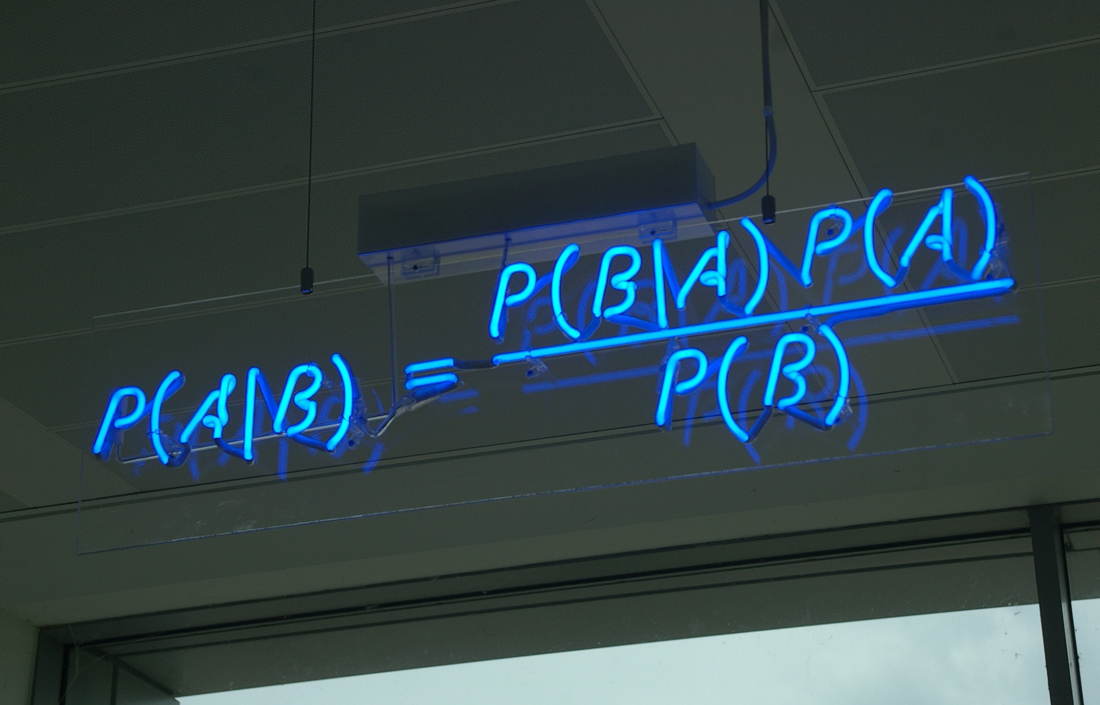
The posterior distribution is equal to the joint distribution divided by the marginal distribution of the evidence.
$$ \color{red}{P(\theta\ |\ \mathcal{D})} = \frac{\color{blue}{P(\mathcal{D}\ |\ \theta)\ P(\theta)}}{\color{green}{P(\mathcal{D})}} = \frac{\color{blue}{P(\mathcal{D}, \theta)}}{\color{green}{\int P(\mathcal{D}\ |\ \theta)\ P(\theta)\ d\theta}} $$For many useful models the marginal distribution of the evidence is hard or impossible to calculate analytically.
Modes of Bayesian Inference
- Conjugate models with closed-form posteriors
- Markov chain Monte Carlo algorithms
- Approximate Bayesian computation
- Distributional approximations
- Laplace approximations, INLA
- Variational inference
Markov Chain Monte Carlo Algorithms
- Construct a Markov chain whose stationary distribution is the posterior distribution
- Sample from the Markov chain for a long time
- Approximate posterior quantities using the empirical distribution of the samples
HTML(mcmc_video)
Beta-Binomial Model
We observe three successes in ten trials, and want to infer the true success probability.
x_beta_binomial = np.array([1, 1, 1, 0, 0, 0, 0, 0, 0, 0])
import pymc3 as pm

with pm.Model() as beta_binomial_model:
    p_beta_binomial = pm.Uniform('p', 0., 1.)
with beta_binomial_model:
    x_obs = pm.Bernoulli('y', p_beta_binomial,
                         observed=x_beta_binomial)
fig

with beta_binomial_model:
    beta_binomial_trace_ = pm.sample(BETA_BINOMIAL_SAMPLES, random_seed=SEED)

beta_binomial_trace = beta_binomial_trace_[BETA_BINOMIAL_BURN::BETA_BINOMIAL_THIN]
fig

Pros
- Asymptotically unbiased: converges to the true posterior afer many samples
- Model-agnostic algorithms
- Well-studied for more than 60 years
Cons
- Can take a long time to converge
- Can be difficult to assess convergence
- Difficult to scale
Variational Inference
- Choose a class of approximating distributions
- Find the best approximation to the true posterior
Variational inference minimizes the Kullback-Leibler divergence
$$\mathbb{KL}(\color{purple}{q(\theta)} \parallel \color{red}{p(\theta\ |\ \mathcal{D})}) = \mathbb{E}_q\left(\log\left(\frac{\color{purple}{q(\theta)}}{\color{red}{p(\theta\ |\ \mathcal{D})}}\right)\right)$$from approximate distributons, but we can't calculate the true posterior distribution.
Minimizing the Kullback-Leibler divergence
$$ \mathbb{KL}(\color{purple}{q(\theta)} \parallel \color{red}{p(\theta\ |\ \mathcal{D})}) = -(\underbrace{\mathbb{E}_q(\log \color{blue}{p(\mathcal{D}, \theta))} - \mathbb{E}_q(\color{purple}{\log q(\theta)})}_{\color{orange}{\textrm{ELBO}}}) + \log \color{green}{p(\mathcal{D})} $$is equivalent to maximizing the Evidence Lower BOund (ELBO), which only requires calculating the joint distribution.
Variational Inference Example
fig

Approximate the true distribution using a diagonal covariance Gaussian from the class
$$\mathcal{Q} = \left\{\left.N\left(\begin{pmatrix} \mu_x \\ \mu_y \end{pmatrix}, \begin{pmatrix} \sigma_x^2 & 0 \\ 0 & \sigma_y^2\end{pmatrix}\ \right|\ \mu_x, \mu_y \in \mathbb{R}^2, \sigma_x, \sigma_y > 0\right)\right\}$$fig

Pros
- A principled method to trade complexity for bias
- Optimization theory is applicable
- Assesment of convergence
- Scalability
Cons
- Biased estimate of the true posterior
- Better for prediction than interpretation
- Model-specific algorithms
Mean field variational inference
Assume the variational distribution factors independently as $q(\theta_1, \ldots, \theta_n) = q(\theta_1) \cdots q(\theta_n)$
The variational approximation can be found by coordinate ascent
$$ \begin{align*} q(\theta_i) & \propto \exp\left(\mathbb{E}_{q_{-i}}(\log(\mathcal{D}, \boldsymbol{\theta}))\right) \\ q_{-i}(\boldsymbol{\theta}) & = q(\theta_1) \cdots q(\theta_{i - 1})\ q(\theta_{i + 1}) \cdots q(\theta_n) \end{align*} $$Coordinate Ascent Cons
- Calculations are tedious, even when possible
- Convergence is slow when the number of parameters is large
Automating Variational Inference in Python
- Maximize ELBO using gradient ascent instead of coordinate ascent
- Tensor libraries calculate ELBO gradients automatically
Common themes
- Monte Carlo estimate of the ELBO gradient
- Minibatch estimates of the joint distribution
BBVI and ADVI arise from different ways of calculating the ELBO gradient

Beta-binomial model
import edward as ed
from edward.models import Bernoulli, Beta, Uniform

ed.set_seed(SEED)

# probability model
p = Uniform(a=0., b=1.)
x_edward_beta_binomial = Bernoulli(p=p)

data = {x_edward_beta_binomial: x_beta_binomial}
# variational approximation
q_p = Beta(a=tf_positive_variable(),
           b=tf_positive_variable())
q = {p: q_p}
%%time
beta_binomial_inference = ed.MFVI(q, data)
beta_binomial_inference.run(n_iter=10000, n_print=None)
fig

from edward.models import PyMC3Model

# probability model
x_beta_binomial_obs = shared(np.zeros(1))

with pm.Model() as beta_binomial_model_untransformed:
    p = pm.Uniform('p', 0., 1., transform=None)
    x_beta_binomial_ = pm.Bernoulli('x', p, observed=x_beta_binomial_obs)

pymc3_data = {x_beta_binomial_obs: x_beta_binomial}
pymc3_beta_binomial_model = PyMC3Model(beta_binomial_model_untransformed)
%%time
# variational distribution
pymc3_q_p = Beta(a=tf_positive_variable(),
                 b=tf_positive_variable())
pymc3_q = {'p': pymc3_q_p}

pymc3_beta_binomial_inference = ed.MFVI(pymc3_q, pymc3_data,
                                        pymc3_beta_binomial_model)
pymc3_beta_binomial_inference.run(n_iter=30000, n_print=None)
fig

Edward-supported modeling "languages"
Direction density calculations
|
Congressional Ideal Points
vote_df.head()
grid.fig

Idea:
- Representatives ($\color{blue}{\alpha_i}$) and bills ($\color{green}{\beta_j}$) each have an ideal point on a spectrum of conservativity
- If a representative's and bill's ideal points are the same, the representative has a 50% chance of voting for the bill
- Bills also have an ability to discriminate ($\color{red}{\gamma_j}$) between conservative and liberal representatives
- Some bills have broad bipartisan support, while some provoke votes along party lines
Representative ideal points
$$ \begin{align*} \color{blue}{\alpha_1}, \ldots, \color{blue}{\alpha_N} & \sim N(0, 1) \end{align*} $$def normal_log_prior(value, loc=0., scale=1.):
return tf.reduce_sum(normal.log_pdf(value, loc, scale))
Bill ideal points and discriminative abilities
$$ \begin{align*} \mu_{\beta} & \sim N(0, 1) \\ \sigma_{\beta} & \sim U(0, 1) \\ \color{green}{\beta_1}, \ldots, \color{green}{\beta_K} & \sim N(\mu_{\beta}, \sigma_{\beta}^2) \end{align*} $$
$$
\begin{align*}
\mu_{\gamma}
& \sim N(0, 1) \\
\sigma_{\gamma}
& \sim U(0, 1) \\
\color{red}{\gamma_1}, \ldots, \color{red}{\gamma_K}
& \sim N(\mu_{\gamma}, \sigma_{\gamma}^2)
\end{align*}
$$
def hierarchical_log_prior(value, mu, sigma):
    log_hyperprior = normal_log_prior(mu) + uniform.log_pdf(sigma, 0., 1.)

    return log_hyperprior + normal_log_prior(value, loc=mu, scale=sigma)
Observation model
$$ \begin{align*} \mathbb{P}(\textrm{Representative }i \textrm{ votes for bill }j\ |\ \color{blue}{\alpha_i}, \color{green}{\beta_j}, \color{red}{\gamma_j}) & = \frac{1}{1 + \exp(-\color{red}{\gamma_j} \left(\color{blue}{\alpha_i} - \color{green}{\beta_j}\right))} \end{align*} $$def log_like(vote, rep, bill, alpha, beta, gamma):
# alpha, beta, and gamma have one entry for representative/bill,
# index them to have one entry per representative/bill combination
alpha_long = long_from_indices(alpha, rep)
beta_long = long_from_indices(beta, bill)
gamma_long = long_from_indices(gamma, bill)
p = tf.sigmoid(gamma_long * (alpha_long - beta_long))
return tf.reduce_sum(bernoulli.logpmf(vote, p))
Edward model
class IdealPoint:
    def log_prob(self, xs, zs):
        """
        xs is a dictionary of observed data
        zs is a dictionary of parameters

        Calculates the model's log joint distribution
        """
        # parameters
        alpha, beta, gamma = zs['alpha'], zs['beta'], zs['gamma']
        mu_beta, mu_gamma = zs['mu_beta'], zs['mu_gamma']
        sigma_beta, sigma_gamma = zs['sigma_beta'], zs['sigma_gamma']

        # observed data
        vote, bill, rep = xs['vote'], xs['bill'], xs['rep']

        # log joint distribution
        log_prior_ = log_prior(alpha,
                               beta, mu_beta, sigma_beta,
                               gamma, mu_gamma, sigma_gamma)
        log_like_ = log_like(vote, rep, bill,
                             alpha, beta, gamma)

        return log_prior_ + log_like_

ideal_point_model = IdealPoint()
BBVI inference
# variational distribution
q_alpha = tf_normal((n_reps,))

q_mu_beta = tf_normal()
q_sigma_beta = tf_uniform()
q_beta = tf_normal((N_BILLS,))

q_mu_gamma = tf_normal()
q_sigma_gamma = tf_uniform()
q_gamma = tf_normal((N_BILLS,))

q = {
    'alpha': q_alpha,
    'beta': q_beta, 'mu_beta': q_mu_beta, 'sigma_beta': q_sigma_beta,
    'gamma': q_gamma, 'mu_gamma': q_mu_gamma, 'sigma_gamma': q_sigma_gamma,
}
%%time
inference = ed.MFVI(q, ideal_point_data, ideal_point_model)
inference.run(n_iter=20000, n_print=None)
fig

Fun project: Recreate the Martin-Quinn dynamic ideal point model for ideology of U.S. Supreme Court justices with Edward

Variational Inference with PyMC3
Automatic Differentiation Variational Inference (ADVI)
- Only applicable to differentiable probability models
- Transform constrained parameters to be unconstrained
- Approximate the posterior for unconstrained parameters with mean field Gaussian
Beta-binomial model
Transformed distributions
fig

%%time
with beta_binomial_model:
    advi_fit = pm.advi(n=20000, random_seed=SEED)
ADVI approxiation to transformed posterior
fig

ADVI approximation to posterior
fig

Dependent Density Regression
fig

Idea: A mixture of linear models, where the unknown number of mixture weights depend on $x$
fig

Mixture weights
The model has infinitely many mixture components, we truncate to $K$
$$ \begin{align*} \alpha_1, \ldots, \alpha_K & \sim N(0, 1) \\ \beta_1, \ldots, \beta_K & \sim N(0, 1) \\ \boldsymbol{\pi} \ |\ \boldsymbol{\alpha}, \boldsymbol{\beta}, x & \sim \textrm{Logit-Stick-Breaking}(\boldsymbol{\alpha} + \boldsymbol{\beta} x) \\ \end{align*} $$K = 20
x_lidar = shared(std_range, broadcastable=(False, True))
with pm.Model() as lidar_model:
alpha = pm.Normal('alpha', 0., 1., shape=K)
beta = pm.Normal('beta', 0., 1., shape=K)
v = tt.nnet.sigmoid(alpha + beta * x_lidar)
pi = pm.Deterministic('pi', stick_breaking(v))
Component linear models
$$ \begin{align*} \gamma_1, \ldots, \gamma_K & \sim N(0, 100) \\ \delta_1, \ldots, \delta_K & \sim N(0, 100) \\ \tau_1, \ldots, \tau_K & \sim \textrm{Gamma}(1, 1) \\ Y_i\ |\ \gamma_i, \delta_i, \tau_i, x & \sim N(\gamma_i + \delta_i x, \tau_i^{-1}) \end{align*} $$with lidar_model:
gamma = pm.Normal('gamma', 0., 100., shape=K)
delta = pm.Normal('delta', 0., 100., shape=K)
tau = pm.Gamma('tau', 1., 1., shape=K)
ys = pm.Deterministic('ys', gamma + delta * x_lidar)
Observation model
$$ \begin{align*} Y\ |\ \boldsymbol{\alpha}, \boldsymbol{\beta}, \boldsymbol{\gamma}, \boldsymbol{\delta}, \boldsymbol{\tau}, x & = \sum_{i = 1}^K \pi_i Y_i \\ \end{align*} $$with lidar_model:
lidar_obs = NormalMixture('lidar_obs', pi, ys, tau,
observed=std_logratio)
ADVI inference
%%time
N_ADVI_ITER = 50000

with lidar_model:
    advi_fit = pm.advi(n=N_ADVI_ITER, random_seed=SEED)
fig

Posterior predictions
PPC_SAMPLES = 5000

lidar_ppc_x = np.linspace(std_range.min() - 0.05,
                          std_range.max() + 0.05,
                          100)

with lidar_model:
    # sample from the variational posterior distribution
    advi_trace = pm.sample_vp(advi_fit, PPC_SAMPLES, random_seed=SEED)

    # sample from the posterior predictive distribution
    x_lidar.set_value(lidar_ppc_x[:, np.newaxis])
    advi_ppc_trace = pm.sample_ppc(advi_trace, PPC_SAMPLES, random_seed=SEED)
Impact of truncation
fig

fig

References
Edward
PyMC3
http://pymc-devs.github.io/pymc3/
PyMC3 port of Probabilistic Programming and Bayesian Methods for Hackers
Variational Inference
Angelino, Elaine, Matthew James Johnson, and Ryan P. Adams. "Patterns of Scalable Bayesian Inference." arXiv preprint arXiv:1602.05221 (2016).
Blei, David M., Alp Kucukelbir, and Jon D. McAuliffe. "Variational inference: A review for statisticians." arXiv preprint arXiv:1601.00670 (2016).
Kucukelbir, Alp, et al. "Automatic Differentiation Variational Inference." arXiv preprint arXiv:1603.00788 (2016).
Ranganath, Rajesh, Sean Gerrish, and David M. Blei. "Black Box Variational Inference." AISTATS. 2014.
Models
Bafumi, Joseph, et al. "Practical issues in implementing and understanding Bayesian ideal point estimation." Political Analysis 13.2 (2005): 171-187.
Fox, Jean-Paul. Bayesian item response modeling: Theory and applications. Springer Science & Business Media, 2010.
Gelman, Andrew, et al. Bayesian data analysis. Vol. 2. Boca Raton, FL, USA: Chapman & Hall/CRC, 2014.
Gelman, Andrew, and Jennifer Hill. Data analysis using regression and multilevel/hierarchical models. Cambridge University Press, 2006.
Ren, Lu, et al. "Logistic stick-breaking process." Journal of Machine Learning Research 12.Jan (2011): 203-239.
Thank You!
@AustinRochford — Monetate Labs
arochford@monetate.com

The Jupyter notebook these slides were generated from is available here