Two Years of Bayesian Bandits for E-Commerce

NYC College of Technology • April, 18 2019 • @AustinRochford
About Me
 |
 |
Chief Data Scientist, Monetate
@AustinRochford • austinrochford.com • github.com/AustinRochford
arochford@monetate.com • austin.rochford@gmail.com
About Monetate

- Founded 2008, web optimization and personalization SaaS
- Observed 5B impressions and $4.1B in revenue during Cyber Week 2017
Non-technical marketer-focused


About this talk
Outline
- Web optimization
- A/B testing
- Multi-armed bandits
- Bayesian bandits
- Thompson sampling
- Bandit bias
- Inverse propensity weighting

A/B testing machinery

|

|

Sequential testing

|

|
Sequential optimization

Multi-armed bandits


Multi-armed bandit systems

Bayesian Bandits

Beta-binomial model
$$ \begin{align*} x_A, x_B & = \textrm{number of rewards from users shown variant } A, B \\ x_A & \sim \textrm{Binomial}(n_A, r_A) \\ x_B & \sim \textrm{Binomial}(n_B, r_B) \\ r_A, r_B & \sim \textrm{Beta}(1, 1) \end{align*} $$
$$ \begin{align*} r_A\ |\ n_A, x_A & \sim \textrm{Beta}(x_A + 1, n_A - x_A + 1) \\ r_B\ |\ n_B, x_B & \sim \textrm{Beta}(x_B + 1, n_B - x_B + 1) \end{align*} $$
Thompson sampling

Thompson sampling randomizes user/variant assignment according to the probabilty that each variant maximizes the posterior expected reward.
The probability that a user is assigned variant A is
$$ \begin{align*} P(r_A > r_B\ |\ \mathcal{D}) & = \int_0^1 P(r_A > r\ |\ \mathcal{D})\ \pi_B(r\ |\ \mathcal{D})\ dr \\ & = \int_0^1 \left(\int_r^1 \pi_A(s\ |\ \mathcal{D})\ ds\right)\ \pi_B(r\ |\ \mathcal{D})\ dr \\ & \propto \int_0^1 \left(\int_r^1 s^{\alpha_A - 1} (1 - s)^{\beta_A - 1}\ ds\right) r^{\alpha_B - 1} (1 - r)^{\beta_B - 1}\ dr \end{align*} $$
Monte Carlo Methods
N = 5000

x, y = np.random.uniform(0, 1, size=(2, N))
fig

in_circle = x**2 + y**2 <= 1
fig

4 * in_circle.mean()
fig

%%time
N_SAMPLES = 10000

a_samples = a_post.rvs(size=N_SAMPLES)
b_samples = b_post.rvs(size=N_SAMPLES)
fig

(a_samples > b_samples).mean()
Thompson sampling, redeemed
- Sample $\hat{r}_A \sim r_A\ |\ n_A, x_A$ and $\hat{r}_B \sim r_B\ |\ n_B, x_B$.
- Assign the user variant A if $\hat{r}_A > \hat{r}_B$, otherwise assign them variant B.
Simulating a bandit
class BetaBinomial:
    def __init__(self, a0=1., b0=1.):
        self.a = a0
        self.b = b0

    def sample(self):
        return sp.stats.beta.rvs(self.a, self.b)

    def update(self, n, x):
        self.a += x
        self.b += n - x
class Bandit:
    def __init__(self, a_post, b_post):
        self.a_post = a_post
        self.b_post = b_post

    def assign(self):
        return 1 * (self.a_post.sample() < self.b_post.sample())

    def update(self, arm, reward):
        arm_post = self.a_post if arm == 0 else self.b_post
        arm_post.update(1, reward)
A_RATE, B_RATE = 0.05, 0.1
N = 1000

rewards_gen = generate_rewards(A_RATE, B_RATE, N)
bandit = Bandit(BetaBinomial(), BetaBinomial())
arms = np.empty(N, dtype=np.int64)
rewards = np.empty(N)

for t, arm_rewards in tqdm(enumerate(rewards_gen), total=N):
    arms[t] = bandit.assign()
    rewards[t] = arm_rewards[arms[t]]

    bandit.update(arms[t], rewards[t])
fig

Simulating many bandits
N_BANDIT = 100

arms = np.empty((N_BANDIT, N), dtype=np.int64)
rewards = np.empty((N_BANDIT, N))

for i in trange(N_BANDIT):
    arms[i], rewards[i] = simulate_bandit(
        generate_rewards(A_RATE, B_RATE, N), N
    )
fig

A/A testing

A/A bandits
N = 2000

arms, rewards = simulate_bandits(
    lambda: generate_rewards(A_RATE, A_RATE, N),
    N, N_BANDIT
)
fig

fig

Why Bayesian?
- Thompson sampling is intuitive and simple to implement
- Principled randomization
- Robustness against delayed feedback
- Marketers are natural Bayesians!

Bandit Bias
fig

fig

fig

Inverse propensity weighting
$$ \hat{r}^{\textrm{IPS}}_A = \frac{1}{n} \sum_{t = 1}^n \frac{Y_i \cdot \mathbb{I}(A_t = 1)}{P(A_t = 1\ |\ \mathcal{D}_{1, t - 1})} $$
where
$$ A_t = \begin{cases} 1 & \textrm{session } t \textrm{ saw variant A} \\ 0 & \textrm{session } t \textrm{ saw variant B} \end{cases}. $$
Calculating $P(A_t = 1\ |\ \mathcal{D}_{1, t - 1})$
ts_fig
%%time
N_MC = 500

a_samples = sp.stats.beta.rvs(
    a_post_alpha[..., np.newaxis],
    a_post_beta[..., np.newaxis],
    size=(N_BANDIT, N, N_MC)
)
b_samples = sp.stats.beta.rvs(
    b_post_alpha[..., np.newaxis],
    b_post_beta[..., np.newaxis],
    size=(N_BANDIT, N, N_MC)
)

a_prob = np.empty((N_BANDIT, N))
a_prob[:, 0] = 0.5
a_prob[:, 1:] = (a_samples > b_samples).mean(axis=2)[:, :-1]
a_ips_est = 1. / plot_t * (rewards * (arms == 0) / a_prob_).cumsum(axis=1)
b_ips_est = 1. / plot_t * (rewards * (arms == 1) / (1 - a_prob_)).cumsum(axis=1)
fig

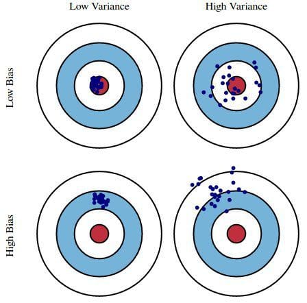
Bias-variance tradeoff
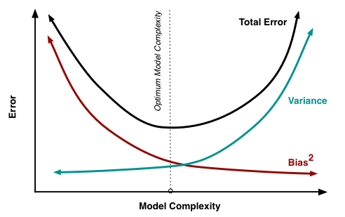
fig

Intuition: the variant with the highest reward rate should receive the most traffic.
fig

Learn more