Utility Theory and Logistic Regression

Logistic regression is perhaps one of the most commonly used tools in all of statistics. While I have mathematically understood and used logistic regression for quite some time, it took me much longer to develop intution for it. It was only a few months ago that I learned about the connection between logistic regression and utility theory.

Suppose a person must decide between two options, \(Y = 0\) or \(Y = 1\). Utility theory posits that each option has an associated utility, \(U_0\) and \(U_1\), respectively. The person chooses the option with the largest utility. My intuition for logistic regression arises from understanding that it arises from a specific utility model.

In logistic regression, we are interested in modeling the effect of a covariate, \(X\), on the person’s choice. In this post, we will work with the logistic regression model

\[\begin{align*} P(Y = 1 | X = x) & = \frac{e^x}{1 + e^x}. \end{align*}\]

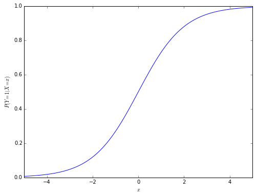
This model is shown graphically below.

from __future__ import division

from matplotlib import pyplot as plt
import numpy as np
from scipy.stats import gumbel_r

def logistic_probability(x):
    exp = np.exp(x)
    
    return exp / (1 + exp)

In terms of utility theory, we assume that each person’s utilities are related to \(X\) by

\[\begin{align*} U_0 | X & = \beta_0 X + \varepsilon_0 \\ U_1 | X & = \beta_1 X + \varepsilon_1 \end{align*}.\]

Here, \(\beta_i X\) represents the observed utility of option \(Y = i\) (\(i = 0, 1\)), and \(\varepsilon_i\) represents btthe random fluctuation in the option’s utility. Logistic regression arises from the assumption that \(\varepsilon_0\) and \(\varepsilon_0\) are independent with Gumbel distributions.

The Gumbel distribution has the density function

\[\begin{align*} f(\varepsilon) & = e^{-\varepsilon}\ \exp(-e^{-\varepsilon}). \end{align*}\]

To show that this utility model gives rise to logistic regression, we see that

\[\begin{align*} P(Y = 1 | X = x) & = P(U_1 > U_0 | X = x) \\ & = P(\beta_1 x + \varepsilon_1 > \beta_0 x + \varepsilon_0) \\ & = P((\beta_1 - \beta_0) x > \varepsilon_0 - \varepsilon_1). \end{align*}\]

It is useful to note that the difference of independent identically distributed Gumbel random variables follows a logistic distribution, so

\[f(\Delta) = \frac{e^{-\Delta}}{(1 + e^{-\Delta})^2},\]

where \(\Delta = \varepsilon_1 - \varepsilon_0\).

Therefore

\[\begin{align*} P(Y = 1 | X = x) & = P((\beta_1 - \beta_0) x > -\Delta) \\ & = \int_{-(\beta_1 - \beta_0) x}^\infty \frac{e^{-\Delta}}{(1 + e^{-\Delta})^2}\ d\Delta. \end{align*}\]

Making the substitution \(t = 1 + e^{-\Delta}\), with \(dt = -e^{-\Delta}\ dt\), we get that

\[\begin{align*} P(Y = 1 | X = x) & = \int_1^{1 + \exp((\beta_1 - \beta_0) x)} t^{-2}\ dt \\ & = \left.t^{-1}\right|_{1 + \exp((\beta_1 - \beta_0) x)}^1 \\ & = 1 - \frac{1}{{1 + \exp((\beta_1 - \beta_0) x)}} \\ & = \frac{{\exp((\beta_1 - \beta_0) x)}}{{1 + \exp((\beta_1 - \beta_0) x)}}. \end{align*}\]

Recalling that

\[\begin{align*} P(Y = 1 | X = x) & = \frac{e^{x}}{1 + e^{x}}, \end{align*}\]

we must have that \(\beta_1 - \beta_0 = 1\).

The fact that there are infinitely many solutions of this equation is a subtle but important point of utility theory, that the difference in utility is both location and scale invariant. We will prove this statement in two parts.

1. For any \(\mu\), let \(\tilde{U}_i = U_i + \mu\) for \(i = 0, 1\). Then \[\begin{align*} \tilde{U_1} - \tilde{U_0} & = U_1 + \mu - (U_0 - \mu) = U_1 - U_0, \end{align*}\] so \(\tilde{U_1} - \tilde{U_0} > 0\) if and only if \(U_1 - U_0 > 0\), and therefore the difference in utility is location invariant.
2. For any \(\sigma > 0\), let \(\tilde{U}_i = \frac{1}{\sigma} U_i\) for \(i = 0, 1\). Then \[\begin{align*} \tilde{U_1} - \tilde{U_0} & = \frac{1}{\sigma}\left(U_1 - U_0\right), \end{align*}\] so \(\tilde{U_1} - \tilde{U_0} > 0\) if and only if \(U_1 - U_0 > 0\), and therefore the difference in utility is scale invariant.

Together, these invariances show that the units of utility are irrelevant, and the only quantity that matters is the difference in utilities. Due to the location invariance in utilities, we may as well set \(\beta_0 = 0\), so \(\beta_1 = 1\) for convenience. Our utility model is therefore

\[\begin{align*} U_0 & = \varepsilon_0 \\ U_1 & = x + \varepsilon_1 \end{align*}.\]

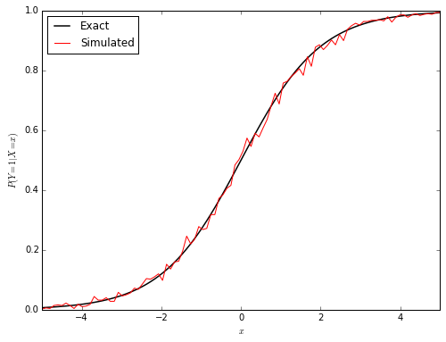
To verify that this utility model is equivalent to logistic regression in a second way, we will simulate \(P(Y = 1 | X = x)\) by generating Gumbel random variables.

N = 500

eps0 = gumbel_r.rvs(size=(N, n))
eps1 = gumbel_r.rvs(size=(N, n))

U0 = eps0
U1 = xs + eps1

simulated_ps = (U1 > U0).mean(axis=0)

The red simulated curve is reasonably close to the black actual curve. (Increasing N would cause the red curve to converge to the black one.)

Aside from being an important tool in econometrics, utility theory helps shed light on logistic regression. The perspective it provides on logistic regression opens the door to generalization and related theories. If the random portions of utility, \(\varepsilon_1\) and \(\varepsilon_0\) are normally distributed instead of Gumbel distributed, the utility model gives rise to probit regression. For a thorough introduction to utility/choice theory, consult the excellent book Discrete Choice Models with Simulation by Kenneth Train, which is freely available online.